IST PVSolar Simulator: Shading and Circuit Analysis Without the Guesswork
Shading is one of the most uncertain inputs in a PV yield estimate, and often one of the most neglected. A designer picks a "far horizon loss" of 1% or 2% by feel, ignores the neighbour's four-storey building, and models a partly shaded string as if every module were equally affected. The energy estimate then carries errors that don't show up until the plant is running.
This update to the IST PVSolar Simulator targets both problems. Site shading is now built automatically from real elevation and building data, and shaded strings are solved with a proper circuit model.
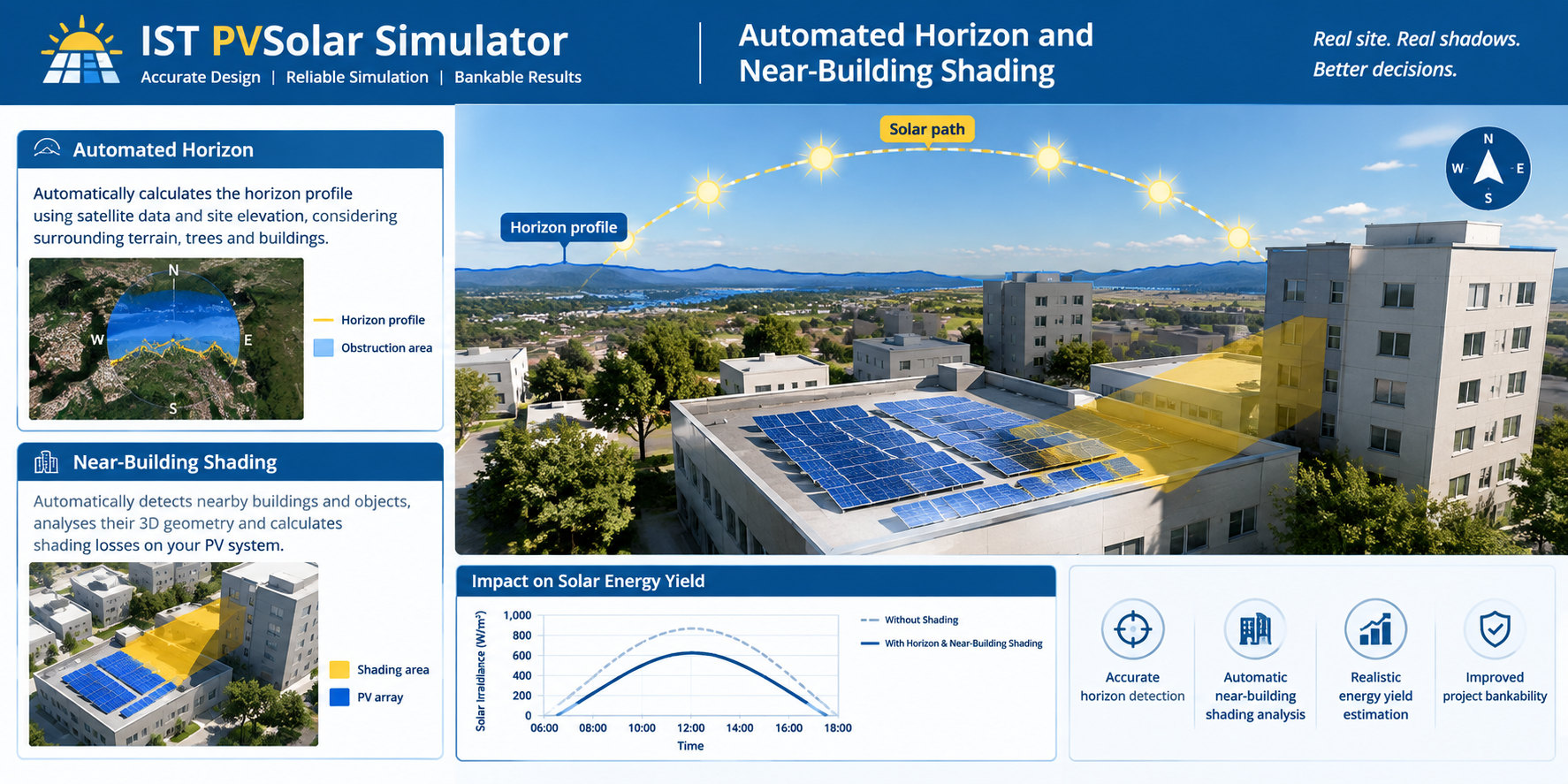
Automated horizon and near-building shading, with no manual input
Enter your site coordinates. The simulator does the rest.
Far horizon from Copernicus DEM
For terrain shading, the simulator builds a horizon profile from the Copernicus DEM (GLO-30/90), the open global elevation dataset from ESA, Airbus and AWS Open Data. For every azimuth bin around the site, it:
- Samples elevation along the line of sight at increasing distances, from about 120 m out to as far as 40 km. The far range is configurable.
- Corrects for Earth's curvature, so distant ridgelines aren't overstated.
- Records the highest angle of obstruction in each direction. That gives the horizon elevation for that compass bearing.
If the DEM lookup fails, the simulator falls back to the PVGIS horizon profile from the EU Joint Research Centre. Your run doesn't stop because one service is unavailable.
Near shading from OpenStreetMap buildings
Terrain isn't the only obstruction. The tower next door matters more than a hill 15 km away. The simulator pulls building footprints within a configurable radius (20 m to 800 m) from OpenStreetMap and turns each one into a shading object:
- Real footprints. Each polygon is reduced to a position, an orientation and a width/depth, so the shadow reflects the building's actual shape and alignment.
- Real heights where they exist. It uses the explicit
heighttag first, then estimates frombuilding:levelsat about 3.2 m per storey. - A sensible default where they don't. Buildings with no height data are assumed to be 9 m, and each one is labelled with where its height came from (tag, levels or default).
- Nearest first. Up to the 80 closest buildings are kept, sorted by distance.
How it feeds the energy model
The horizon profile is applied hour by hour in the simulation:
- Beam irradiance is cut off whenever the sun's elevation falls below the interpolated horizon elevation at the sun's azimuth. A hill that blocks the low winter sun only removes beam energy when it actually blocks it.
- Diffuse sky-view loss is calculated from the whole profile, since a raised horizon also cuts the sky the array can see.
Every result carries a provenance line naming the terrain and building sources. Reviewers and lenders can see where the data came from instead of taking it on trust.
Per-module Kirchhoff series/parallel circuit solver
Most simulators handle partial shading with an aggregate performance factor: shade about 10% of an array, lose about X%. That works for annual estimates, but it hides what happens inside a mismatched string.
The new circuit solver works at module level. It solves the actual Kirchhoff circuit for a named list of modules, each with its own diode parameters and its own irradiance and temperature. Those values can come straight from a per-module shading or CAD layout.
Series strings
In a series string, one current flows through every module and the string voltage is the sum of the module voltages at that current. The solver:
- Computes each module's voltage at a given current from its single- or two-diode model.
- Clamps reverse-biased modules at the bypass-diode drop, so a badly shaded module behaves like a real one with a bypass diode instead of collapsing the string.
- Scans the full current range and refines the peak. Mismatched strings can have several local maxima, and a simple hill-climb can lock onto the wrong one.
- Returns the string's true Pmp, Vmp, Imp and Voc, plus the voltage of every module at the operating point. A module driven into bypass conduction shows up immediately.
Parallel arrays
When several strings share one DC bus or MPPT, the solver finds the current of each string at a common bus voltage and sums them. It then locates the true maximum of the combined P(V) curve. This captures the cost of a common design mistake: combining strings of different length, orientation or shading on one MPPT input. The array result comes with a per-string breakdown, so you can see which string is dragging the others down.
What it makes possible
- Exact string and array diagnostics for a specific shading pattern, such as a chimney shadow on one row, rather than a generic derate.
- MLPE comparison. The optimizer and microinverter model uses the same solver for the string case, so a string inverter and module-level electronics are compared against a real circuit result.
- Wiring-diagram insight. Per-module voltages show which modules are back-fed and where the losses occur.
- API access. The solver is exposed as a service, so it can be called from your own workflows.
One note on the word "exact": the circuit solution is exact for the diode model it is given. The result is only as good as the module parameters behind it, which is why the simulator fits them from datasheet data.
Together, these changes move shading analysis from an assumption you defend to a calculation you can show. That helps at design review, in a bankability report, and when the plant's measured output has to be explained against the model.