Dynamic Solar Yield Simulation using IST PVSolar Simulator

How to Perform a Dynamic Solar Yield Simulation Using IST PVSolar Simulator

Most PV design tools let you run a quick monthly estimate — twelve numbers in, a rough annual yield out. IST PVSolar Simulator's dynamic simulation mode does something different: it runs the plant hour-by-hour (or even in 15-minute sub-hourly steps) through a full physics chain — sun position, spectral losses, cell temperature, diode I-V behavior, and true inverter clipping — instead of applying flat empirical de-rates. Here's how to actually run one.

In Step 7 of the workflow, you choose a Time Resolution: Monthly (12 values, fast what-if), Hourly (8,760 steps), or Sub-hourly (35,040 steps, 15-minute). Monthly mode is useful for quick sanity checks. Hourly and sub-hourly are what you want for a bankable report — they trace the exact sun path, Perez (1990) sky-diffuse transposition, Martin-Ruiz incidence-angle losses, air-mass spectral correction, and Faiman cell-temperature modeling for every single timestep of the year.

Step 1 — Site and weather data

Start with project and site details, then the part that actually feeds the dynamic engine: importing an hourly weather dataset. You have three real options:

PVGIS TMY — an ISO 15927-4 Typical Meteorological Year with measured beam-normal DNI

NASA Hourly TMY — a typical year built from NASA POWER's hourly climatology (2005–2024 by default)

Manual entry for a named bankable-grade source (Meteonorm, SolarGIS, SolarAnywhere) if your lender or independent engineer requires it

If you skip this and don't import a TMY, the hourly engine will still run — it derives a deterministic hourly series from your monthly averages — but a real TMY import is what gives you a genuinely bankable, source-attributed result.

Step 2 — Orientation

Set tilt and azimuth (or use Auto-Optimize Tilt, which sweeps 0–60° at your fixed azimuth and locks in whatever maximizes annual POA). This single choice — the "Orientation Loss vs Optimum" figure — is often the largest yield lever in the whole design, since every other loss downstream is applied on top of whatever irradiance this step delivers to the array.

Step 3–5 — Modules, inverters, and strings

Pick your module and inverter, verify the string-voltage window against your site's winter/summer design temperatures, then build at least one sub-array (modules per string, strings per MPPT, inverters). This is the minimum required to run any simulation — economics is optional and can be excluded from the final report entirely.

Step 6 — Losses and (optional) economics

Step 4's loss table — thermal, soiling, spectral, LID, mismatch, wiring, IAM — feeds directly into the dynamic run. If you want a full bankability picture, Step 6 adds CAPEX/OPEX/financing and can later drive the Monte-Carlo financial risk engine.

Step 7 — Choosing dynamic resolution and running

Here's the actual dynamic step: set Time Resolution to Hourly or Sub-hourly, and pick a PV Cell Model (single-diode, two-diode, or linear temperature-coefficient — single-diode is the default and most widely validated). Then hit Run.

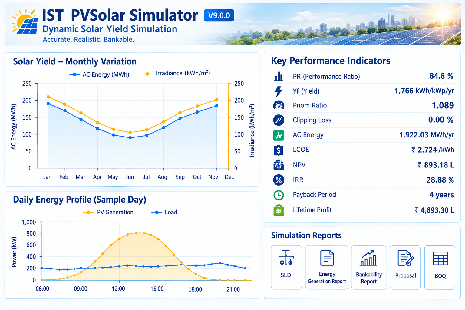
You get DC kWp, annual E_AC, Performance Ratio, Specific Yield (Yf), a full monthly breakdown, P50/P75/P90/P95 probability curves, a 25-year revenue forecast, and CO₂ savings. One thing worth knowing in advance: a hot, sunny month can post a lower PR than a cloudy monsoon month — because PR normalizes out irradiance and measures conversion efficiency, and hotter cells are less efficient. That's correct physics, not a bug.

Every run is also auto-logged in a per-project batch table, so you can sweep tilt, module, inverter, or string count and compare KPIs side-by-side without losing earlier attempts — useful for finding your actual optimum design rather than your first guess.

Use high-resolution imagery for the actual layout

Before you get to Step 7, the 3D Shadow Analysis tool is where the physical layout gets built. You upload a drone orthomosaic (JPG/PNG/GeoTIFF), with optional GeoJSON/KML boundary files or a LAS/LAZ point cloud for extra precision. A built-in ✨ Enhance Image (AI, 2x) step sharpens and doubles resolution entirely in-browser. Once the image is scaled against a known real-world distance, you trace roof faces or ground-mount parcels and let ⚡ Auto Fit place panels across each traced area, combining results automatically when a site mixes multiple roof faces and ground parcels.

Assisted shading detection, not autonomous layout

Worth being precise here: the tool includes genuine AI-assisted tree detection in the Mark Tool (it flags likely obstructions — trees, buildings, chimneys, poles — for you to confirm), plus a Shadow Scan that reads visibly darker regions in the photo itself and flags any panel sitting under one. That's real, useful automation for shading. But the layout itself — roof tracing, panel placement, string configuration — stays a guided, human-in-the-loop process with live electrical safety checks at every step, not something an autonomous agent designs unsupervised. For a bankable report, that's arguably the right trade-off: a lender's independent engineer wants a traceable, human-reviewed layout, not a black-box one.

From layout to report: the full run

Once a traced layout exists, ✔ Apply Shading Loss to Simulation writes the computed loss percentage into Step 4, and — where available — feeds a real hourly shading profile and real bifacial geometry (pitch, GCR, mounting height) into the Step 7 run, replacing the generic row-shading formula with your exact site. From there, Generate Report pulls the Row Pitch Diagram, Sun Path Chart, Areas Breakdown, and a 3D Site Preview snapshot straight into the PDF, alongside the KPI tables and probability curves from the dynamic run itself.

Where the "AI" in AI/ML actually sits

The software does have a dedicated AI & Machine Learning module, but it's worth describing accurately rather than as a buzzword. It's a set of lightweight, fully transparent models — ordinary least squares with ridge regularization — trained client-side on your own simulated hourly dataset: energy prediction, PR modeling, fault/anomaly z-scores, a soiling-and-cleaning-schedule optimizer, and simple weather forecasting. Nothing leaves the browser, and the documentation is upfront that these models learn the simulator's own physics, so they're positioned for methodology research and teaching — real field decisions should still rely on monitored data. That transparency (you can see the regression coefficients, R², and RMSE for every model) is a more defensible feature for a bankability-focused tool than an opaque black-box "AI agent" would be.

Benefits that actually improve accuracy and efficiency

The genuine efficiency gains come from a few concrete places: the Suggest Optimum Simulation step, which reviews every batch run client-side and recommends a configuration weighing yield, financial, and bankability outcomes together rather than yield alone; the AI/ML PR & Yield recommendation engine, which turns the Step 4 loss table into prioritized, estimated-impact actions instead of leaving you to interpret it manually; and the Research tab's model-characterization suite (thermal model comparison, inverter behavior, shading-model comparison, SCADA benchmarking against real measured data) — which is what actually validates the simulation's accuracy against ground truth, rather than assuming it.

Customize the financial analysis

Step 6 lets you configure CAPEX and OPEX line items, financing terms, discount rate, tariff escalation, and a choice of depreciation method (WDV or SLM, with India-specific additional depreciation under Section 32(1)(iia)). That feeds both a project-level financial model and an equity-level bankability view, plus an hourly-Perez-driven Monte-Carlo financial risk run that reports DSCR/LLCR and IRR/NPV as P10–P95 distributions rather than single point estimates — the kind of sensitivity range a lender's due-diligence review actually asks for.

The honest version of "AI-powered"

It's tempting to market a tool like this as a fully AI-driven design assistant. The more accurate story is narrower and, for a bankability-focused product, arguably better: targeted machine-learning and image-processing features — tree detection, image enhancement, PR/yield recommendations, batch-run optimization — sit around a transparent, standards-referenced physics engine , rather than replacing it. The physics stays auditable; the AI layer just helps you interpret and improve what the physics engine already computed.